Projections and Distance
Projection is a fundamental operation in linear algebra that maps vectors onto subspaces. This document covers orthogonal projection, vector decomposition, and distance calculations—essential tools for understanding geometric relationships between points, vectors, and lines.
Orthogonal Projection Concept
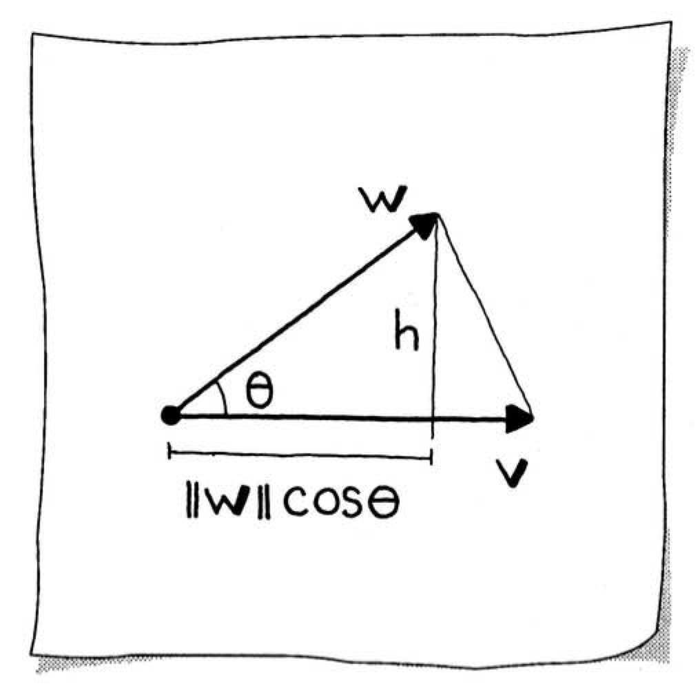
Orthogonal projection acts like sunlight casting shadows at a right angle. When we project a vector $\mathbf{w}$ onto another vector $\mathbf{v}$, we find the component of $\mathbf{w}$ that lies in the direction of $\mathbf{v}$.
Geometric Interpretation
The projection of $\mathbf{w}$ onto $\mathbf{v}$ creates a "footprint" of length $b = \lVert\mathbf{w}\rVert \cos(\theta)$, derived from basic trigonometry where $\cos(\theta) = b / \text{hypotenuse}$. The orthogonal projection vector $\mathbf{u}$ is this length multiplied by the unit vector in the direction of $\mathbf{v}$:
\[\mathbf{u} = \left(\lVert\mathbf{w}\rVert \cos(\theta)\right) \frac{\mathbf{v}}{\lVert\mathbf{v}\rVert} = \frac{\mathbf{v} \cdot \mathbf{w}}{\lVert\mathbf{v}\rVert^2} \mathbf{v}\]
This result follows from the relationship between the dot product and cosine established earlier.
Projection Notation
Sometimes this projection is expressed as:
\[\mathbf{u} = \operatorname{proj}_{\mathcal{V}_1} \mathbf{w}\]
where $\mathcal{V}_1$ is the set of all 2D vectors $k\mathbf{v}$, referred to as a one-dimensional subspace of $\mathbb{R}^2$. The projection $\mathbf{u}$ is the best approximation to $\mathbf{w}$ in the subspace $\mathcal{V}_1$.
Dot Product and Projection
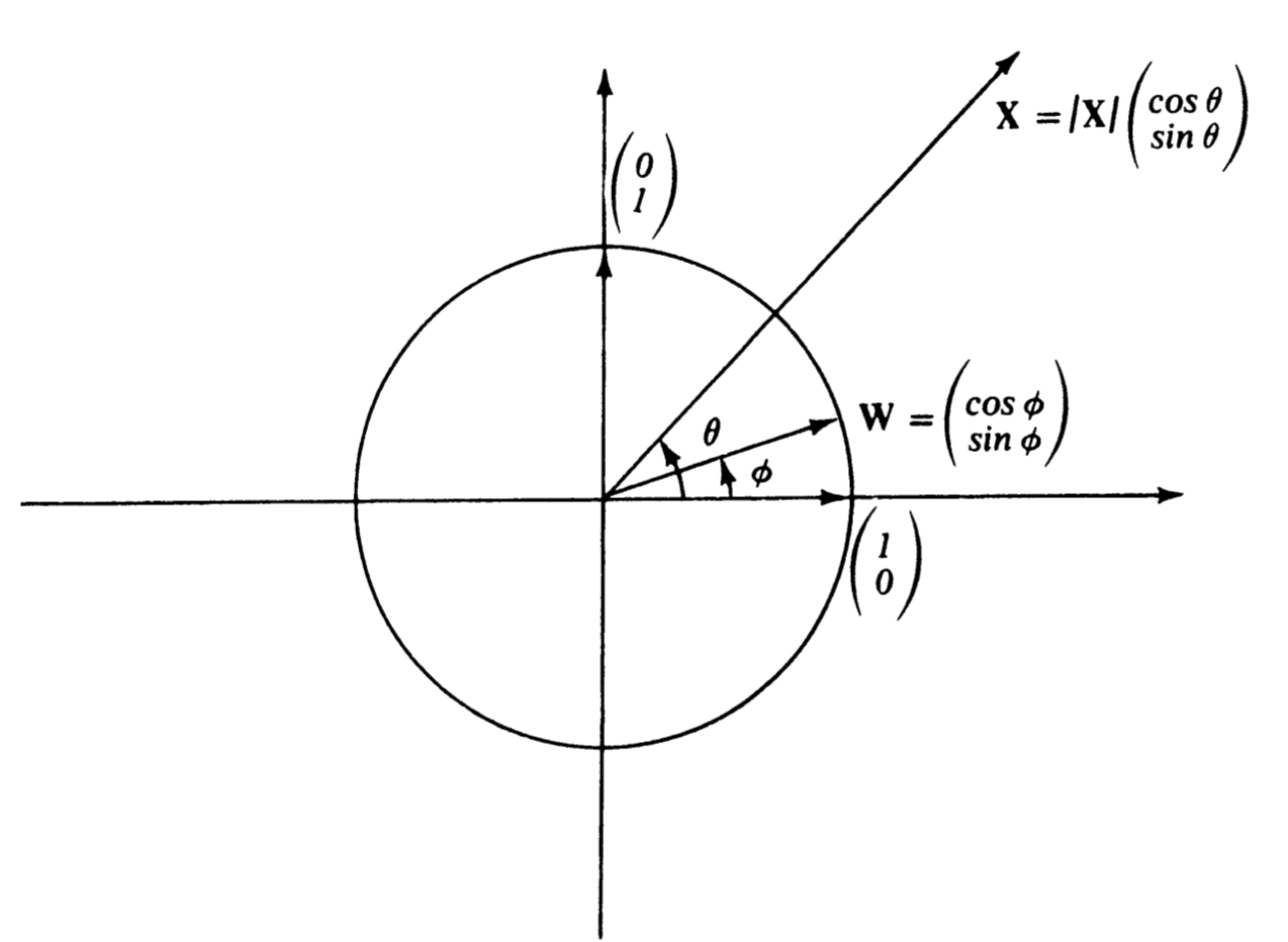
For any vector $\mathbf{X} = \lbrack x, y \rbrack^T$, the dot product with the unit vector $\mathbf{E}_1 = \lbrack 1, 0 \rbrack^T$ gives:
\[\mathbf{X} \cdot \mathbf{E}_1 = x\]
Thus, the dot product of $\mathbf{X}$ with a unit vector is the coordinate of the projection of $\mathbf{X}$ to that axis.
More generally, for any unit vector $\mathbf{W} = \lbrack \cos\phi, \sin\phi \rbrack^T$ and a vector $\mathbf{X} = \lvert\mathbf{X}\rvert \lbrack \cos\theta, \sin\theta \rbrack^T$ in polar form, we have:
\[\mathbf{X} \cdot \mathbf{W} = \lvert\mathbf{X}\rvert \cos(\theta - \phi)\]
Therefore, the dot product of a vector $\mathbf{X}$ with a unit vector $\mathbf{W}$ equals the product of the length of $\mathbf{X}$ and the cosine of the angle between them.
Projection Formula
Projection onto a Unit Vector
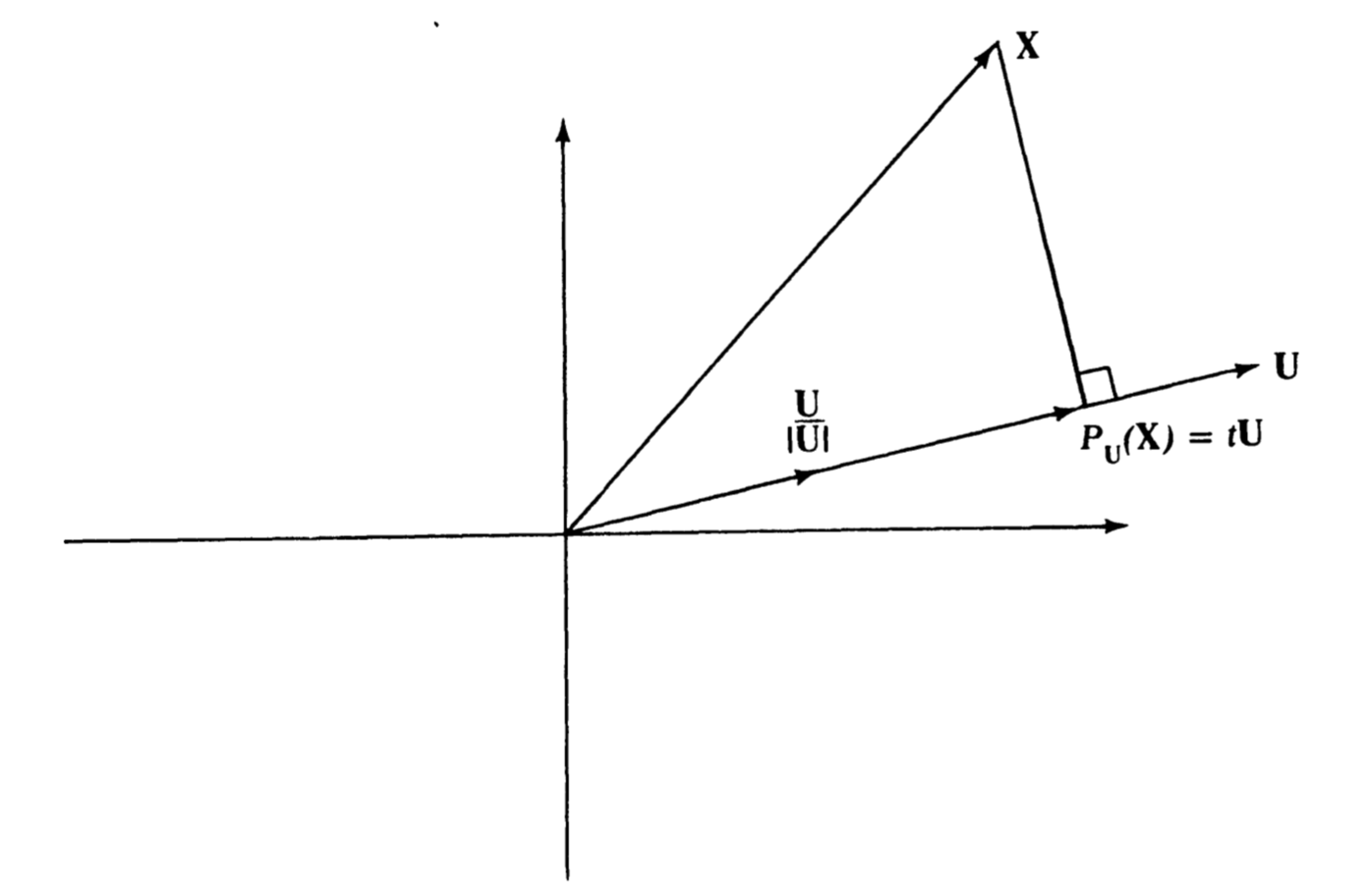
If $\mathbf{W}$ is a unit vector, then the projection of $\mathbf{X}$ onto the line through the origin in direction $\mathbf{W}$ is:
\[P_{\mathbf{W}}(\mathbf{X}) = (\mathbf{X} \cdot \mathbf{W})\mathbf{W}\]
Projection onto an Arbitrary Vector
For an arbitrary nonzero vector $\mathbf{U}$, we first normalize it, then project:
\[P_{\mathbf{U}}(\mathbf{X}) = \left(\mathbf{X} \cdot \frac{\mathbf{U}}{\lvert\mathbf{U}\rvert}\right) \frac{\mathbf{U}}{\lvert\mathbf{U}\rvert} = \frac{(\mathbf{X} \cdot \mathbf{U})\mathbf{U}}{\lvert\mathbf{U}\rvert^2} = \frac{(\mathbf{X} \cdot \mathbf{U})\mathbf{U}}{(\mathbf{U} \cdot \mathbf{U})}\]
The equivalence of $\lVert\mathbf{v}\rVert^2$ and $\mathbf{v} \cdot \mathbf{v}$ can be verified:
julia> using LinearAlgebra

julia> v = [2, 2]
2-element Vector{Int64}:
 2
 2

julia> Int(round(norm(v)^2)) == dot(v, v)
true
Length of the Projection
The length of the projection of $\mathbf{X}$ onto the line along $\mathbf{U}$ is:
\[\left\lvert\mathbf{X} \cdot \frac{\mathbf{U}}{\lvert\mathbf{U}\rvert}\right\rvert = \frac{\lvert\mathbf{X} \cdot \mathbf{U}\rvert}{\lvert\mathbf{U}\rvert}\]
julia> w = [0, 2]
2-element Vector{Int64}:
 0
 2

julia> v = [2, 2]
2-element Vector{Int64}:
 2
 2

julia> u = orthproj(v, w)  # projection of w onto v
2-element Vector{Int64}:
 1
 1

# Verify: length of projection equals formula
julia> isapprox(norm(u), abs(dot(w, v)) / norm(v), rtol=1e-15)
true
Alternative Derivation
We can find the projection by seeking a scalar $t$ such that $\mathbf{X} - t\mathbf{U}$ is orthogonal to $\mathbf{U}$:
\[0 = (\mathbf{X} - t\mathbf{U}) \cdot \mathbf{U} = (\mathbf{X} \cdot \mathbf{U}) - t(\mathbf{U} \cdot \mathbf{U})\]
Solving for $t$:
\[t = \frac{\mathbf{X} \cdot \mathbf{U}}{\mathbf{U} \cdot \mathbf{U}}\]
Therefore:
\[P_{\mathbf{U}}(\mathbf{X}) = t\mathbf{U} = \left(\frac{\mathbf{X} \cdot \mathbf{U}}{\mathbf{U} \cdot \mathbf{U}}\right)\mathbf{U}\]
Worked Example
To find the projection of $\mathbf{B} = \lbrack 1, 2 \rbrack^T$ onto the line along $\mathbf{A} = \lbrack 3, 1 \rbrack^T$:
\[P_{\mathbf{A}}(\mathbf{B}) = \left(\frac{\mathbf{A} \cdot \mathbf{B}}{\mathbf{A} \cdot \mathbf{A}}\right)\mathbf{A} = \frac{5}{10}\mathbf{A} = \frac{1}{2}\mathbf{A} = \begin{bmatrix} \frac{3}{2} \\ \frac{1}{2} \end{bmatrix}\]
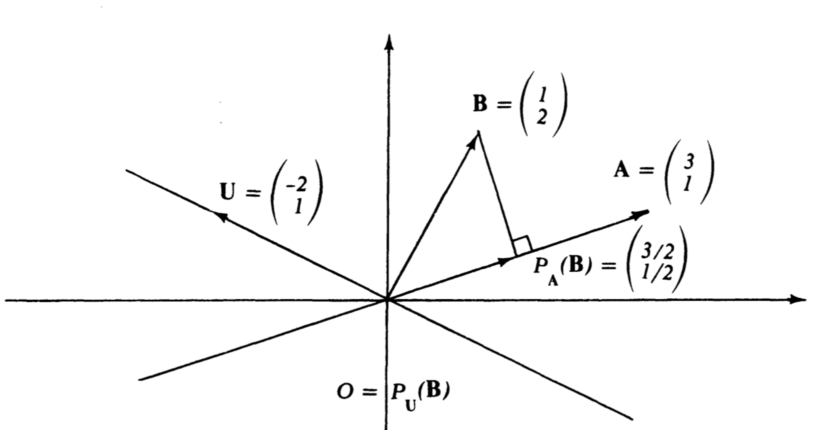
When projecting $\mathbf{B} = \lbrack 1, 2 \rbrack^T$ onto $\mathbf{U} = \lbrack -2, 1 \rbrack^T$:
\[P_{\mathbf{U}}(\mathbf{B}) = \left(\frac{\mathbf{B} \cdot \mathbf{U}}{\mathbf{U} \cdot \mathbf{U}}\right)\mathbf{U} = \frac{0}{5}\mathbf{U} = \mathbf{0}\]
This confirms our intuition: if $\mathbf{X}$ is orthogonal to $\mathbf{U}$, the projection is the zero vector (the origin).
Orthogonal Decomposition
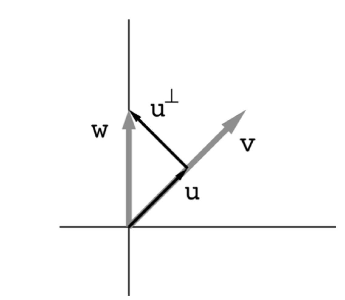
Using orthogonal projection, any 2D vector $\mathbf{w}$ can be decomposed into a sum of two perpendicular vectors:
\[\mathbf{w} = \mathbf{u} + \mathbf{u}^{\perp}\]
where $\mathbf{u}$ is the projection onto $\mathbf{v}$ and $\mathbf{u}^{\perp}$ is the component orthogonal to $\mathbf{v}$.
Computing the Orthogonal Component
Having found $\mathbf{u}$, the orthogonal component is:
\[\mathbf{u}^{\perp} = \mathbf{w} - \frac{\mathbf{v} \cdot \mathbf{w}}{\lVert\mathbf{v}\rVert^2}\mathbf{v} = \mathbf{w} - \operatorname{proj}_{\mathcal{V}_1}\mathbf{w}\]
Thus $\mathbf{u}^{\perp}$ is formed by subtracting from $\mathbf{w}$ its component in the direction of $\mathbf{u}$.
Julia Implementation
using LinearAlgebra

function orthproj(v::Vector, w::Vector)
    u = (dot(v, w) / norm(v)^2) * v
    [round(Int, x) for x in u]
end
Example:
julia> v = [2, 2]
2-element Vector{Int64}:
 2
 2

julia> w = [0, 2]
2-element Vector{Int64}:
 0
 2

julia> u = orthproj(v, w)
2-element Vector{Int64}:
 1
 1

julia> ut = w - u       # component of w orthogonal to u
2-element Vector{Int64}:
 -1
  1

julia> u + ut           # verify decomposition: reconstructs w
2-element Vector{Int64}:
 0
 2
Projection Matrix
To construct a 2D orthogonal projection matrix, choose a unit vector $\mathbf{u}$ defining the line onto which to project. The matrix columns are the projections of the standard basis vectors $\mathbf{e}_1$ and $\mathbf{e}_2$ onto $\mathbf{u}$:
\[\begin{aligned} \mathbf{a}_1 &= \frac{\mathbf{u} \cdot \mathbf{e}_1}{\lVert\mathbf{u}\rVert^2}\mathbf{u} = u_1\mathbf{u} \\ \mathbf{a}_2 &= \frac{\mathbf{u} \cdot \mathbf{e}_2}{\lVert\mathbf{u}\rVert^2}\mathbf{u} = u_2\mathbf{u} \end{aligned}\]
The projection matrix is:
\[A = \lbrack u_1\mathbf{u} \quad u_2\mathbf{u} \rbrack = \frac{\mathbf{u}\mathbf{u}^T}{\lVert\mathbf{u}\rVert^2}\]
This dyadic matrix has rank 1, reflecting that projections reduce dimensionality.
Properties of Projection Matrices
A projection matrix is idempotent: $A = AA$. Geometrically, once a vector has been projected onto a line, applying the same projection leaves the result unchanged.
function projection_matrix(u::Vector)
    u * transpose(u) ./ (transpose(u) * u)
end
julia> u = [1, 2]
2-element Vector{Int64}:
1
2
julia> A = projection_matrix(u)
2×2 Matrix{Float64}:
0.2 0.4
0.4 0.8
julia> v = [1, 2]
2-element Vector{Int64}:
1
2
julia> v′ = A * v
2-element Vector{Float64}:
1.0
2.0
julia> A * v′ # Idempotent: projecting again gives same result
2-element Vector{Float64}:
1.0
2.0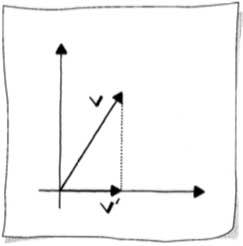
Distance from a Point to a Line
If you have a point $\mathbf{r}$ and a line $\mathbf{l}$, the distance from the point to the line is the length of the perpendicular segment. This is the shortest distance, as established by the orthogonal projection concept.
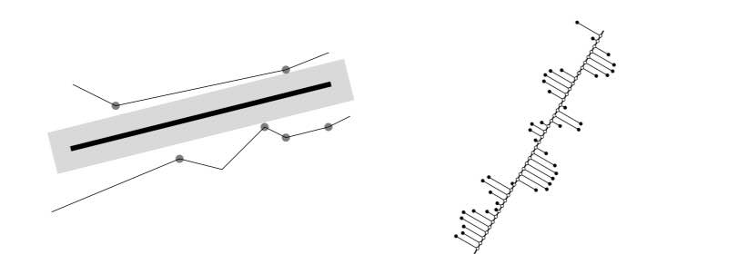
There are two main approaches depending on the line representation:
Using the Parametric Equation
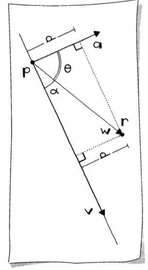
Given: A line $\mathbf{l}$ in parametric form, defined by point $\mathbf{p}$ and direction vector $\mathbf{v}$, and a point $\mathbf{r}$.
Find: The distance $d(\mathbf{r}, \mathbf{l})$.
Solution: Form the vector $\mathbf{w} = \mathbf{r} - \mathbf{p}$ and use:
\[d = \lVert\mathbf{w}\rVert \sin(\alpha)\]
where $\sin(\alpha) = \sqrt{1 - \cos^2(\alpha)}$ and:
\[\cos(\alpha) = \frac{\mathbf{v} \cdot \mathbf{w}}{\lVert\mathbf{v}\rVert\lVert\mathbf{w}\rVert}\]
function distance_to_parametric_line(p::Point, v::Vector, r::Point)
    w = Vector(r - p)
    cosα = dot(v, w) / (norm(v) * norm(w))
    d = norm(w) * sqrt(1 - cosα^2)
end
julia> p = Point(0, 4)
julia> v = [2, -4]
julia> r = Point(5, 3)
julia> distance_to_parametric_line(p, v, r)
4.024922359499621Using the Implicit Equation
Given: A line $\mathbf{l}$ in implicit form $ax + by + c = 0$ and a point $\mathbf{r}$.
Find: The distance $d(\mathbf{r}, \mathbf{l})$.
Solution: With the normal vector $\mathbf{a} = \lbrack a, b \rbrack^T$:
\[d = \frac{ar_1 + br_2 + c}{\lVert\mathbf{a}\rVert}\]
Or in vector notation:
\[d = \frac{\mathbf{a} \cdot (\mathbf{r} - \mathbf{p})}{\lVert\mathbf{a}\rVert}\]
where $\mathbf{p}$ is any point on the line.
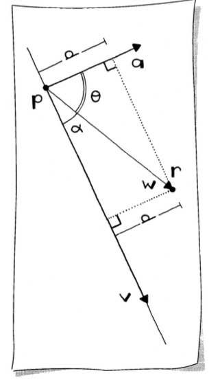
Derivation: The implicit equation is derived from the dot product $\mathbf{a} \cdot (\mathbf{x} - \mathbf{p}) = 0$. For a point $\mathbf{r}$ not on the line:
\[v = \mathbf{a} \cdot (\mathbf{r} - \mathbf{p}) = \mathbf{a} \cdot \mathbf{w} = \lVert\mathbf{a}\rVert\lVert\mathbf{w}\rVert\cos(\theta)\]
From the right triangle geometry, $\cos(\theta) = d / \lVert\mathbf{w}\rVert$, so:
\[v = \lVert\mathbf{a}\rVert d \implies d = \frac{v}{\lVert\mathbf{a}\rVert}\]
function distance_to_implicit_line(a::Number, b::Number, c::Number, r::Point)
    v = [a, b]
    d = ((a * r[1]) + (b * r[2]) + c) / norm(v)
end
julia> a, b, c = 4, 2, -8
julia> r = Point(5, 3)
julia> distance_to_implicit_line(a, b, c, r)
4.024922359499621Point Normal Form
When checking many points against a line, it's efficient to store the line in point normal form where $\lVert\mathbf{a}\rVert = 1$, eliminating the division:
\[\frac{ax_1 + bx_2 + c}{\lVert\mathbf{a}\rVert} = 0\]
function implicit_line_point_normal_form(a::Number, b::Number, c::Number)
    v = [a, b]
    n = norm(v)
    (a/n, b/n, c/n)
end
Foot of a Point on a Line
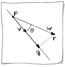
The foot of a point $\mathbf{r}$ on a line is the point $\mathbf{q}$ on the line closest to $\mathbf{r}$—where the perpendicular from $\mathbf{r}$ meets the line.
Given: A line $\mathbf{l}$ in parametric form (point $\mathbf{p}$ and vector $\mathbf{v}$) and a point $\mathbf{r}$.
Find: The point $\mathbf{q}$ on the line closest to $\mathbf{r}$.
Solution: Since $\mathbf{q}$ lies on the line:
\[\mathbf{q} = \mathbf{p} + t\mathbf{v}\]
We need to find $t$. From the geometry, with $\mathbf{w} = \mathbf{r} - \mathbf{p}$:
\[\cos(\theta) = \frac{\lVert t\mathbf{v}\rVert}{\lVert\mathbf{w}\rVert}\]
Using the dot product formula for cosine:
\[\cos(\theta) = \frac{\mathbf{v} \cdot \mathbf{w}}{\lVert\mathbf{v}\rVert\lVert\mathbf{w}\rVert}\]
Solving for $t$:
\[t = \frac{\mathbf{v} \cdot \mathbf{w}}{\lVert\mathbf{v}\rVert^2}\]
function foot_of_line(p::Point, v::Vector, r::Point)
    w = Vector(r - p)
    t = dot(v, w) / norm(v)^2
    q = Point(p + t * v)
end
julia> p = Point(0, 1)
julia> v = [0, 2]
julia> r = Point(3, 4)
julia> foot_of_line(p, v, r)
2-element Point{2, Float64}:
0.0
4.0
julia> r = Point(2, -1)
julia> foot_of_line(p, v, r)
2-element Point{2, Float64}:
0.0
-1.0Distance from Foot to Line Point
In some applications, the signed distance from $\mathbf{q}$ to $\mathbf{p}$ is needed:
\[\lVert\mathbf{q} - \mathbf{p}\rVert = \lVert t\mathbf{v}\rVert = t\lVert\mathbf{v}\rVert = \frac{\mathbf{v} \cdot \mathbf{w}}{\lVert\mathbf{v}\rVert}\]
function foot_of_line(p::Point, v::Vector, r::Point)
    w = Vector(r - p)
    t = dot(v, w) / norm(v)^2
    q = Point(p + t * v)
    d = dot(v, w) / norm(v)
    (q, d)
end
julia> r = Point(3, 4)
julia> foot_of_line(p, v, r)
([0.0, 4.0], 3.0)
julia> r = Point(2, -1)
julia> foot_of_line(p, v, r)
([0.0, -1.0], -2.0)Side of a Line
The distance formula from the implicit equation provides more than just the magnitude—its sign indicates which side of the line a point lies on.
Given an implicit line $ax + by + c = 0$ with normal vector $\mathbf{a} = \lbrack a, b \rbrack^T$:
\[d = \frac{ar_1 + br_2 + c}{\lVert\mathbf{a}\rVert}\]
The sign of $d$ depends on the orientation of $\mathbf{a}$:
- Positive $d$: The point is on the side toward which $\mathbf{a}$ points
- Negative $d$: The point is on the opposite side
- Zero $d$: The point is on the line
function point_side_of_line(p::Point, q::Point, x::Point)
    a = q[2] - p[2]
    b = p[1] - q[1]
    c = -(a * p[1]) - (b * p[2])
    (a * x[1] + b * x[2] + c) / norm([a, b])
end
julia> p = Point(2, 2)
julia> q = Point(6, 4)
# Point on the line
julia> x = Point(2, 2)
julia> point_side_of_line(p, q, x)
0.0
# Point on opposite side from normal direction
julia> x = Point(0, 3)
julia> point_side_of_line(p, q, x)
-1.7888543819998317
# Point on same side as normal direction
julia> x = Point(4, 1)
julia> point_side_of_line(p, q, x)
0.8944271909999159This is useful for determining whether points are separated by a line, or for classifying points relative to geometric boundaries.
Area of a Parallelogram
The parallelogram formed by two vectors has an area that can be computed using the projection formula.
Formula Derivation
For a parallelogram with one vertex at the origin and adjacent vertices at $\mathbf{A} = \lbrack a, c \rbrack^T$ and $\mathbf{B} = \lbrack b, d \rbrack^T$:
The height is the distance from $\mathbf{A}$ to the line along $\mathbf{B}$:
\[h = \frac{\lvert ad - bc\rvert}{\sqrt{b^2 + d^2}}\]
Multiplying by the base length $\sqrt{b^2 + d^2}$:
\[\text{Area} = \lvert ad - bc\rvert\]
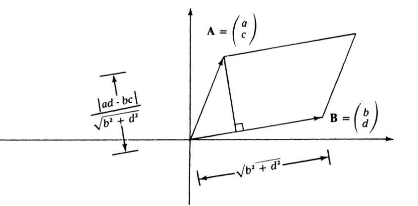
This expression $\lvert ad - bc\rvert$ is the absolute value of the determinant of the matrix $\lbrack\mathbf{A} \; \mathbf{B}\rbrack$.
Using Foot of Point
A more elegant approach uses the foot-of-point calculation:
function parallelogram_area(P::Point, A::Point, B::Point)
    v = Vector(B - P)
    w = Vector(A - P)
    t = dot(v, w) / norm(v)^2
    q = Point(P + t * v)
    d = dot(v, w) / norm(v)
    area = d * norm(v)
    (q, d, area)
end
julia> A = Point(3, 1)
julia> B = Point(1, 3)
julia> P = Point(0, 0)
julia> parallelogram_area(P, A, B)
([0.6, 1.8], 1.897..., 6.0)
# Verify with determinant formula
julia> (A[1] * B[2]) - (B[1] * A[2])
8
julia> abs((A[1] * B[2]) - (B[1] * A[2]))
8Summary
| Concept | Formula | Key Insight |
|---|---|---|
| Orthogonal projection | $\frac{(\mathbf{v} \cdot \mathbf{w})}{\lVert\mathbf{v}\rVert^2}\mathbf{v}$ | Best approximation in subspace |
| Orthogonal decomposition | $\mathbf{w} = \mathbf{u} + \mathbf{u}^{\perp}$ | Any vector splits into parallel and perpendicular parts |
| Distance (parametric) | $\lVert\mathbf{w}\rVert\sin(\alpha)$ | Uses sine of angle |
| Distance (implicit) | $\frac{ar_1 + br_2 + c}{\lVert\mathbf{a}\rVert}$ | Sign indicates side |
| Foot of point | $\mathbf{p} + t\mathbf{v}$ where $t = \frac{\mathbf{v} \cdot \mathbf{w}}{\lVert\mathbf{v}\rVert^2}$ | Closest point on line |
| Parallelogram area | $\lvert ad - bc\rvert$ | Absolute value of determinant |